If you read Australian election coverage or previews, you will likely be familiar with the classic two-party pendulum – where government and opposition seats are lined up on opposite sides and ordered by their margin. An example from the Wikipedia page for the 2022 South Australian state election is included below:
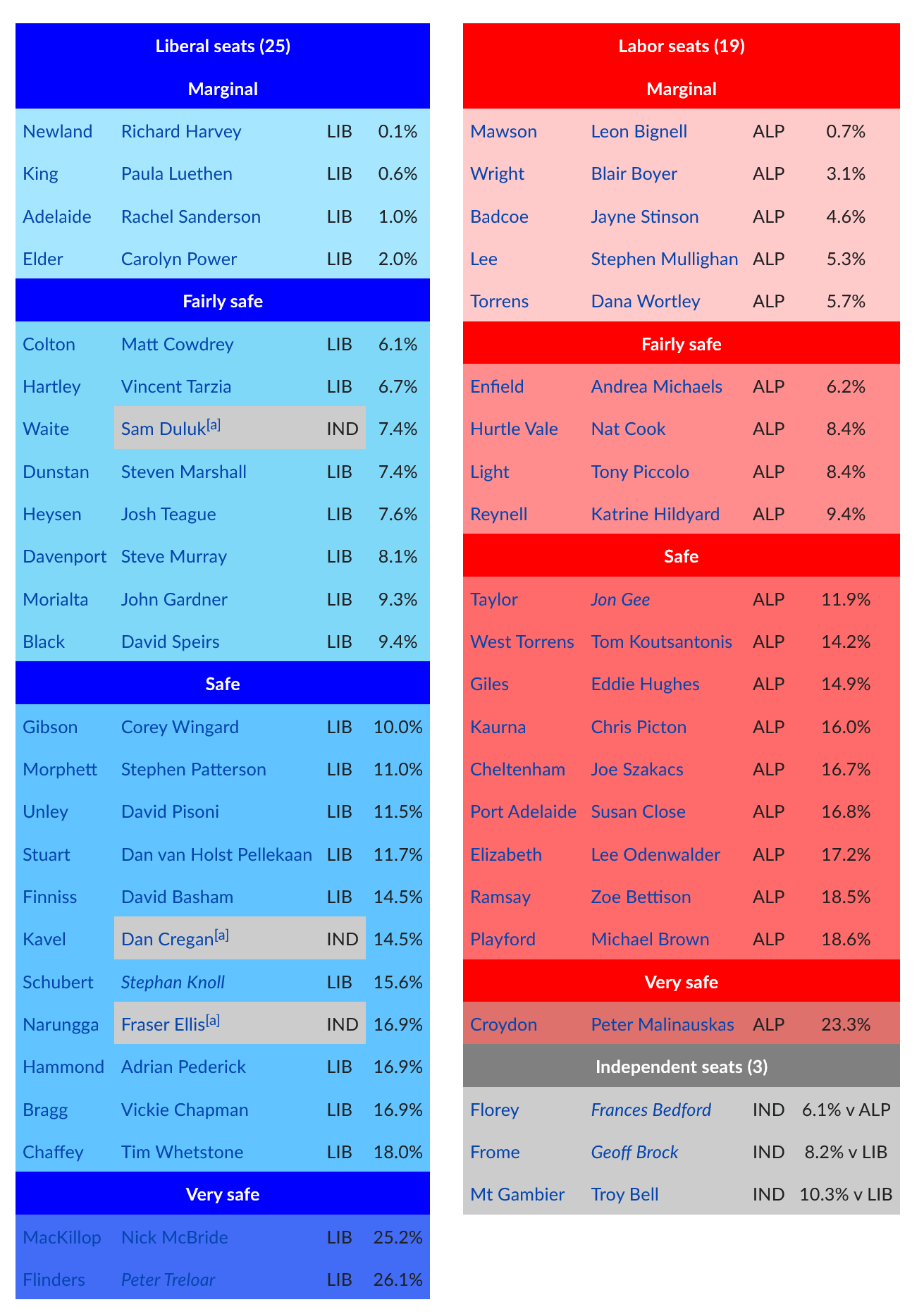
When/if polling for the election comes in, the two-party-preferred (2pp) swing from the polling is projected onto the pendulum, with certain seats “predicted” to fall if the poll is right. For example, if there was a 2% swing to Labor, this model would “predict” that Newland, King, Adelaide and Elder would flip to Labor.
However, no swing is ever fully uniform, and hence seat totals are better forecasted by conditional probability models which assume that the swing is random and uneven. In such a model, seats wins are treated as probabilities rather than win/lose outcomes; for example, in the 2% swing to Labor scenario, Elder would be treated as being Labor-held 50% of the time and Liberald-held the other 50% (instead of being “Labor win” or “Liberal win”). Dr Bonham has constructed one such model for the upcoming federal election, and we’ve previously found that such models have a fairly good predictive track record.
However, I’m not here today to discuss the conditional probability model. Instead, I want to focus on the central assumption behind uniform swing modelling, which is that the best way to estimate the “expected” two-party-preferred (2pp) for each electorate is to apply a uniform swing onto the last 2pp recorded in that electorate. Taking Elder (Liberal 52%) as an example, if there’s a statewide swing of 2% to Labor, this means Elder is expected to end up with an average 50% 2pp (with some margin of error depending on how uneven swings are expected to be throughout the state).
First off – let’s see how well a probabilistic model based on a uniform swing fares, if it “knows” what the 2pp result will be ahead of time. Below are some seat totals from a conditional probability model applied to federal elections (where more data is available), compared to the actual seat total at each election:
Uniform swing probabilistic models are fairly accurate at forecasting seat totals
(Note that the below seat forecasts were made using the actual election results, NOT final polling)
| Election | Predicted Labor seats, uniform swing | Actual Labor seats | Difference |
|---|---|---|---|
| 1993 | 82.2 | 80 | -2.2 |
| 1996 | 54.3 | 49 | -5.4 |
| 1998 | 71.4 | 67 | -4.7 |
| 2001 | 65.1 | 65 | -0.1 |
| 2004 | 59 | 60 | 1 |
| 2007 | 81.5 | 83 | 1.5 |
| 2010 | 75.7 | 72 | -3.7 |
| 2013 | 58 | 55 | -3 |
| 2016 | 66.5 | 69 | 2.5 |
| 2019 | 67.6 | 68 | 0.4 |
| Average difference | ± 2.5 |
| Election | Predicted Coalition seats, uniform swing | Actual Coalition seats | Difference |
|---|---|---|---|
| 1993 | 63.8 | 65 | 1.2 |
| 1996 | 92.7 | 94 | 1.3 |
| 1998 | 72.6 | 80 | 6.4 |
| 2001 | 81.9 | 83 | 1.1 |
| 2004 | 88 | 87 | -1 |
| 2007 | 66.5 | 65 | -1.5 |
| 2010 | 71.3 | 73 | 2.7 |
| 2013 | 89 | 90 | 1 |
| 2016 | 79.5 | 76 | -3.5 |
| 2019 | 77.4 | 77 | -0.4 |
| Average difference | ± 2.0 |
(Remember that the above seat totals were forecasted knowing what the final 2pp result would be. A uniform swing model which relied on polling would obviously produce larger errors, however the purpose of this piece is to find out how best to translate vote shares into seat forecasts, not on the issue of polling error.)
If a uniform swing model is given the correct 2pp result ahead of time, it’ll be able to get the seat totals for the major parties to within +/- 2 to 3 seats on average. Obviously, this will change if the combined major party vote collapses, but it’s worth noting that these models have been fairly accurate so far despite the sustained rise in the non-Labor/Coalition vote.
However, this does not mean that the accuracy of the forecasted 2pp for each seat can’t be improved. A good example is adjusting for candidate effects – where some voters support a candidate (usually an incumbent) but would not otherwise support a generic candidate from that party. On average this is worth about a point on the 2pp for major-party incumbents; adjusting swings for this effect can improve the accuracy of a uniform swing forecast:
Adjusting for candidate effects improves two-party-preferred uniform swing forecasts
| Election | Avg. uniform swing error | Avg. uniform swing error (adjusted for candidate effects) |
|---|---|---|
| 1993 | 2.78 | 2.87 |
| 1996 | 3.06 | 2.85 |
| 1998 | 3.91 | 2.39 |
| 2001 | 1.9 | 1.86 |
| 2004 | 2.3 | 2.26 |
| 2007 | 2.3 | 2.2 |
| 2010 | 3.32 | 2.25 |
| 2013 | 2.27 | 2.33 |
| 2016 | 2.39 | 2.38 |
| 2019 | 3 | 3.07 |
| Average | 2.7 | 2.4 |
On average, adjusting for candidate effects reduces the average 2pp error from 2.7% to 2.4%. While that might not sound like a lot, this amounts to an 11% reduction in the average error, an improvement which is larger for elections which follow elections with large seat swings (e.g. 1998, 2010).
Are there any other avenues to improving the accuracy of uniform swing forecasts? Well, the most common method of improving any kind of estimate is to combine multiple measurements (i.e. averaging). While there is no way to “measure” the 2-party lean of an electorate at an election multiple times, one way of conducting “multiple” measurements could be to combine the 2-party lean of an electorate from several elections. This idea has precedent in other contexts – in their US election forecasts, FiveThirtyEight generally uses data from the last two elections as opposed to simply relying on the last election’s results.
However, one can easily imagine how such an approach might have its flaws. First off, in some cases electorates “re-align” or get significantly altered by demographic change, producing long-term shifts in an electorate’s left/right lean. In such a scenario, using data from older elections would only make things worse, as your forecast would be permanently “behind the curve” on such realignments.
Secondly, unlike US presidential elections – which are conducted using unchanging state boundaries, Australian electorates are regularly redistributed. This introduces an extra source of error – any inaccuracies in making post-redistribution estimates are likely to be greater when attempting to produce estimates for two elections prior.
As usual, though, talk is cheap, and numbers are worth their exponents in gold. So let’s try combining the 2-party lean (for a start, we’ll define it as Electorate’s Coalition 2pp – Nationwide Coalition 2pp) from two prior elections to see if that improves the uniform swing forecast. To begin with, I’m going to assume that the 2-party lean from one election back (e.g. the 2-party lean from 2016, used to forecast the electorate’s result in 2019) is twice as important as the 2-party lean from two elections back (e.g. the 2-party lean from 2013, used to forecast the electorate’s result in 2019), but we’ll check this assumption as we go.
So the formula for an electorate’s 2-party-preferred is:
Electorate 2pp = (2*(Two-party lean, last election) + (Two-party lean, two elections back))/3 + National 2pp
I produced some rough 2pp estimates for federal elections, using the below methodology. It’s not super important, just know that the error on the two-elections-back redistribution estimates here are likely higher than they would be for, say, Antony Green’s estimates.
Firstly, data on the two-party-preferred by polling place and electorate was downloaded from the relevant Australian Electoral Commission (AEC) Tally Room.
If the electorate had not been redistributed for two elections, then estimates were simply produced by subtracting the swing estimates provided by the AEC from the election result.
For example, the Northern Territory (NT) was not redistributed between 2008 and 2017. Hence, for the 2016 election, the estimates for NT electorates were produced by simply subtracting the 2013 and 2016 swings from the result.
Declaration votes (e.g. postal and pre-poll votes) were then “allocated” to polling-places. This was estimated on the following basis:
- The gap between declaration votes and ordinary votes were calculated for each electoral division. For example, in Eden-Monaro 2013, the Liberals won 50.34% of the 2pp in ordinary votes, and 51.59% of the 2pp in declaration votes, so declaration votes would be expected to favour the Liberals by 1.25%.
- This gap was then applied to the 2pp in each polling place. For example, in Bega 2013 (polling place in Eden-Monaro), the Liberal 2pp in the on-the-day vote was 39.86%, so the Liberal 2pp in declaration votes which would have otherwise gone to Bega was estimated to be (39.86% + 1.25%) = 41.11%. For polling places where voters came from different electoral divisions, a weighted average of the declaration vote gap was calculated using the % of voters from each electoral division.
- The number of declaration votes “allocated” to each polling place was estimated on the basis of the % of the on-the-day vote cast at each polling place. Continuing with the example of Bega, in 2013, 1533 of 37639 votes in Eden-Monaro were cast at Bega, or about 4.1% of the ordinary vote. As 6475 declaration votes were cast across Eden-Monaro, (0.041 * 6475) = 263.7 declaration votes were estimated to have originated from voters living near Bega.
- The estimated 2pp in declaration votes from each polling place was used to estimate the “number” of 2pp votes for each side. With Bega 2013, that means an estimated 108.4 declaration votes would be Liberal 2pp, and an estimated 155.3 declaration votes would have been Labor 2pp. These votes were then added onto the pile for that polling place.
Polling places were then “allocated” to each division. As a first pass, any polling place inside a particular electoral division was “allocated” to said electoral division; however if a polling-place was close to the border between two electoral divisions, its vote would be “split” using the closest-straight-line distance to the other electorate and a regression on distance vs % of voters from each electoral division.
For each electoral division, the 2pp vote for each side was added up from the polling place data. A 2pp was calculated and compared to the nationwide 2pp (obtained by summing all redistributed electorates’ estimated 2pps) to obtain a 2-party lean estimate for each division.
For electorates from one election back (e.g. the 2016 estimates of 2pp for each division, to be used for predicting the 2019 election), the AEC estimates were used. To do so, the estimated swing for each electoral division published by the AEC was subtracted from the estimated 2pp result (i.e. the 2016-to-2019 swing was subtracted from the 2019 result to get the 2016 estimate).
Like I mentioned above, this is a very rough method (the votes-by-SA1 method that Ben Raue and others use is more precise). For the purposes of getting a rough estimate of 2-party lean it’s probably fine, but of course if you had a more precise method of estimating 2pp by electorate from two elections back you would get more accurate forecasts.
Combining two-party lean estimates from two elections appears to reduce forecast error
| Election | 2pp error, Uniform swing | 2pp error, Combined-lean uniform swing |
|---|---|---|
| 2010 | 3.32 | 2.79 |
| 2013 | 2.27 | 1.81 |
| 2016 | 2.39 | 2.41 |
| 2019 | 3.01 | 2.7 |
| Average | 2.7 | 2.4 |
First off – this is a very small sample size (n = 4) and hence I would be cautious about drawing too many conclusions solely from this sample. Nevertheless, combining two-party lean estimates from the last two elections, as opposed to simply using the last election result, appears to improve forecast error by a similar degree as adjusting for candidate effects. This is in spite of the higher error likely associated with my rough method of estimating margins for two elections back – a more accurate method (like the SA1 method) would produce more accurate estimates.
It’s worth noting that this was also something we saw in our WA 2021 forecast – switching to using the 2-party lean from just the last election (as opposed to two elections back) increased the 2-party-preferred error by 0.1% from 4.04% to 4.14%. (yes, this SMBC comic is how a lot of forecasting feels like)
What about my assumption that the 2-party lean from one election back was about twice as important as the 2-party lean from two elections back? Turns out that’s not too far off the mark – here’s a graph comparing the amount of weight given to the 2-party lean from two elections back to the average error:

The “ideal” weight for 2-party leans in backtesting is 37% two elections back, and 63% last election. This isn’t a huge improvement over a simple 1:2 (i.e. 33% to 67%) weighting – the average error goes down from 2.428% to 2.427%, an “improvement” which may easily be due to noise. Hence, I’d recommend – and have used – the simple 1:2 weight (last election is twice as important as two elections back) for estimating electorates’ 2-party leans.
How does this apply to the South Australian state election?
First, let’s apply this model to a South Australian state election to see if it continues to produce improvements at the state level. These redistributions take a lot of time and effort (thanks Rebekah!) and hence I’ve opted to just perform one backtest on the 2018 SA state election:
(if you’re on a mobile device, scroll right for full data or turn your device landscape. Click the Previous and Next buttons to view all data.)
| District | Abs. error, uniform swing | Abs. error, combined-lean uniform swing |
|---|---|---|
| Adelaide | 0.9 | 1.6 |
| Badcoe | 0.3 | 1.1 |
| Black | 7.5 | 8.6 |
| Bragg | 1.4 | 0.1 |
| Chaffey | 5.6 | 6.6 |
| Cheltenham | 2.6 | 1.2 |
| Colton | 5.1 | 4.6 |
| Croydon | 2.1 | 3.2 |
| Davenport | 0.4 | 0.6 |
| Dunstan | 3.6 | 2.4 |
| Elder | 1.4 | 2.1 |
| Elizabeth | 5.5 | 4.1 |
| Enfield | 1.2 | 1.4 |
| Finniss | 2.2 | 2.7 |
| Flinders | 1.5 | 0.7 |
| Florey | 0.8 | 0.3 |
| Frome | 1.1 | 1.9 |
| Gibson | 6.7 | 6.3 |
| Giles | 8.9 | 7.9 |
| Hammond | 3.8 | 2.8 |
| Hartley | 5.8 | 5.6 |
| Heysen | 2.7 | 3.6 |
| Hurtle Vale | 2.9 | 2 |
| Kaurna | 4.6 | 4.4 |
| Kavel | 2.1 | 1.6 |
| King | 1.8 | 1.3 |
| Lee | 1.2 | 0.4 |
| Light | 4.8 | 4.9 |
| MacKillop | 0.6 | 0.2 |
| Mawson | 3.4 | 3.8 |
| Morialta | 0.4 | 0.2 |
| Morphett | 3.7 | 4 |
| Mount Gambier | 1.8 | 0.1 |
| Narungga | 4.4 | 3.3 |
| Newland | 2.9 | 2.9 |
| Playford | 3.5 | 3.4 |
| Port Adelaide | 1.7 | 1.4 |
| Ramsay | 0.1 | 0.6 |
| Reynell | 2.3 | 2.1 |
| Schubert | 3.1 | 1.4 |
| Stuart | 4.1 | 6.9 |
| Taylor | 1.2 | 0.8 |
| Torrens | 1 | 0.2 |
| Unley | 3.5 | 2.4 |
| Waite | 1.2 | 2 |
| West Torrens | 0.2 | 0.5 |
| Wright | 0.9 | 0.8 |
| Average error | 2.73 | 2.57 |
(2014 rough estimates on 2022 boundaries available here)
This is a similar improvement to what we found at the 2021 WA state election – a 0.16% reduction in the average error (or a relative 5.9% reduction in error size). Of course, we should avoid generalising from such small sample sizes, but it is entirely possible that combining two elections’ data is less useful at the state level, with fewer voters per electorate (more randomness).
But what does this mean for the upcoming SA state election?
Some of you may have noticed that our forecast is predicting surprisingly high odds for Labor to flip certain “Fairly safe” Liberal seats, such as Colton and Hartley. Using the statewide 2pp currently predicted by our model (Liberal 44.9%), our forecast expects a few of these seats to be more Labor-leaning than a uniform swing:
| District | 2pp predicted by uniform swing | 2pp predicted by forecast (16/Mar/2022) | Difference |
|---|---|---|---|
| Colton | 49.1% | 46.9% | -2.2% |
| Hartley | 49.7% | 47.4% | -2.3% |
| Waite | 50.4% | 51.4% | +1.0% |
| Dunstan | 50.4% | 51.5% | +1.1% |
| Heysen | 50.6% | 53.3% | +2.7% |
| Davenport | 51.1% | 49.2% | -1.9% |
| Morialta | 52.3% | 51.5% | -0.8% |
| Black | 52.4% | 48.8% | -3.6% |
So what’s going on? Well, our forecast takes a bit more than just the last two elections into account, but for starters, here’s my estimates of the Liberal 2pp for the 2014 and 2018 elections on each district’s 2022 boundaries:
| District | 2014 estimate | 2018 estimate | Combined 2-party lean |
|---|---|---|---|
| Colton | 52.9% | 56.6% | +3.1% |
| Hartley | 53.0% | 57.1% | +4.5% |
| Waite | 57.8% | 57.1% | +5.1% |
| Dunstan | 56.4% | 57.5% | +4.9% |
| Heysen | 62.3% | 57.5% | +6.8% |
| Davenport | 56.6% | 57.0% | +4.6% |
| Morialta | 58.8% | 59.5% | +7.0% |
| Black | 53.3% | 59.6% | +5.2% |
| Statewide 2pp | 53.0% | 51.9% |
You might be starting to see a pattern here. The seats where the model expects Labor to do better than a uniform swing would – Colton, Hartley, Davenport and Black – are seats which sat a lot closer to the statewide 2pp before sharply swinging right in 2018. A similar factor explains Heysen – used to be a fair bit more Liberal-leaning than it used to.
Allow me to put this into a visual format. Here’s the plot of our 2pp estimates for Colton going back five elections compared to the statewide 2pp, with the 2018 result circled in black:

Here’s Black – I’m sure you can work out which result is 2018:

(A similar plot for Hartley is already up on the how-our-model-works page. 2018 isn’t circled on there, but I’m sure you can guess which one it is by now.)
What if you don’t trust my redistribution estimates? That’s fine – let’s have a look at the 2014-to-2018 swing in each electorate on their 2018 boundaries – tables from each district’s Wikipedia page, and keep in mind there was a 1.1% statewide swing to Labor in 2018:
Let’s start with Colton:
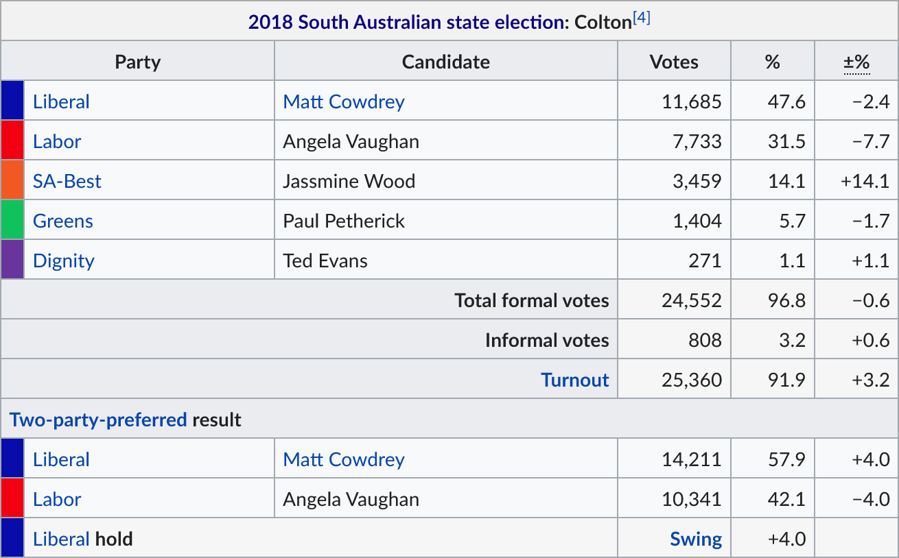
On its old boundaries, Colton had a Liberal 2pp of 53.9% in 2014, which put it fairly in-line with the state as a whole (Liberal 2pp, 53.0%). It was only in 2018 that it suddenly shifted sharply towards the Liberals.
Now, onto Hartley:
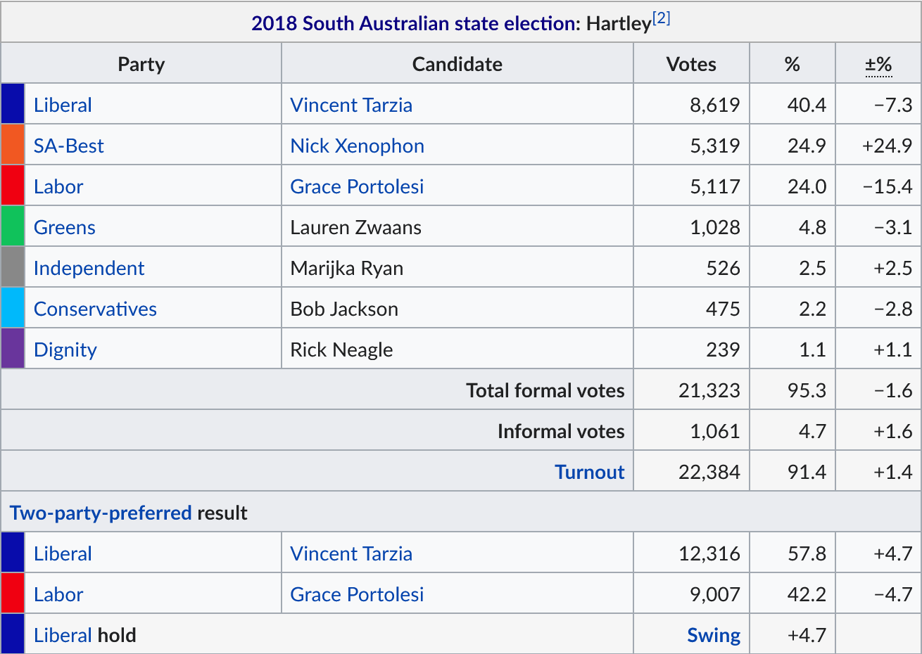
A similar situation – 2018 Hartley used to sit at 53.1% Liberal 2pp, matching up nearly perfectly with the state. Again, its shift to the Liberals in 2018 was unusually sharp and out of line with its history of tacking fairly close to the statewide vote. This may have had something to do with the candidacy of Nick Xenophon (SA Best’s former leader), who out-polled Labor but failed to win the seat.
The swing in the district of Black is even more extreme:
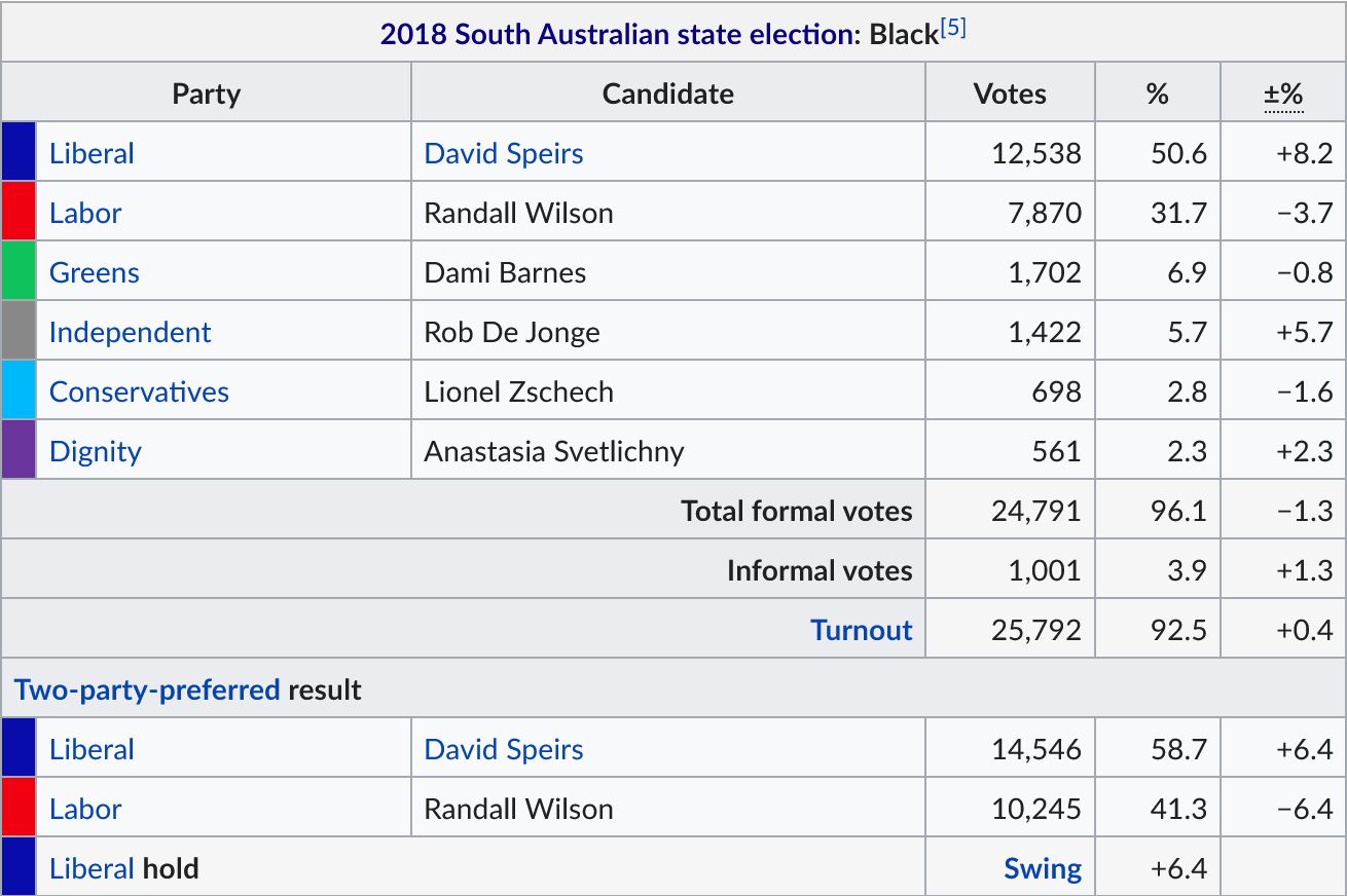
Before 2018, Black (on its old boundaries) would have had a Liberal 2pp of just 52.3%, making it very very slightly to the left of the state. The 2020 redistribution likely shifted this around somewhat (bumping Black up from Liberal 58.7% to Liberal 59.4%), but it still wouldn’t be enough for 2022 Black to be a “fairly safe Liberal” seat in 2014.
It’s also worth noting that while our model expects these seats to be less Liberal-leaning on average than at the last election, there is still a very real chance that they will become more Liberal-leaning. For each electorate, our model estimates that there’s anywhere from a 1 in 6 (Black) to a 1 in 3 (Davenport) that the district will lean further to the right than in 2018, for an overall 2 in 3 chance that at least one of these electorates (Colton, Hartley, Davenport, Black) will be more conservative-leaning than in 2018.
In other words – given their history, I’d expect these electorates to revert somewhat towards the centre at the upcoming election. But it’s entirely possible that we’re seeing a permanent realignment of these areas into the Liberal church, and I wouldn’t go around betting my last dollar on them reverting.
Overall, how does this impact the upcoming state election?
It means that Labor may have a few backup options that aren’t readily visible on a simple pendulum, and that Labor might have a better shot at a majority than what a uniform swing would assign them.
Looking at an electorate’s broader history of voting, rather than just focusing on the last election, appears to produce more accurate forecasts. While we only have a small sample size of elections to test on, the effect is fairly consistent and appears to be replicated overseas, suggesting that the improvement is genuine.
Applying this approach to the upcoming SA state election, we find that several seats with a seemingly-large Liberal lean have much more moderate histories. If history holds, Colton, Hartley and Black give Labor a few backup options for a majority in the event of they fail to win any of the Liberal marginal seats. Collectively, they play the role of Arizona/Florida/North Carolina/Georgia for this election – possibly giving the centre-left an alternate path to a majority should it fall flat in more seemingly-marginal electorates. However, much like Florida in the 2020 US presidential election, it’s likely that at least one of these electorates is going to be more conservative-leaning than it was at the last election; hence Labor would be ill-advised to pin its hopes on any one district reverting.
(Of course, there are similar seats on the other end of the pendulum, as well as some Liberal marginals (Newland, King, Elder) where we expect the Liberals to somewhat out-perform a uniform swing. However, as it looks like there’s going to be a swing to Labor, the probabilities in those electorates aren’t going to differ much from simple uniform swing unless the Liberals manage to keep the popular vote very close.)
Edit: I’ve added a follow-up to this piece, where I use Australian state voting patterns to examine whether shifts in electorate 2-party lean – e.g. Colton shifting right in 2018 – will continue instead of revert)